An introduction to Big O in Swift

Big O notation. It's a topic that a lot of us have heard about, but most of us don't intuitively know or understand what it is. If you're reading this, you're probably a Swift developer. You might even be a pretty good developer already, or maybe you're just starting out and Big O was one of the first things you encountered while studying Swift.

Regardless of your current skill level, by the end of this post, you should be able to reason about algorithms using Big O notation. Or at least I want you to understand what Big O is, what it expresses, and how it does that.

Understanding what Big O is

Big O notation is used to describe the performance of a function or algorithm that is applied to a set of data where the size of that set might not be known. This is done through a notation that looks as follows: O(1).

In my example, I've used a performance that is arguably the best you can achieve. The performance of an algorithm that is O(1) is not tied to the size of the data set it's applied to. So it doesn't matter if you're working with a data set that has 10, 20 or 10,000 elements in it. The algorithm's performance should stay the same at all times. The following graph can be used to visualize what O(1) looks like:

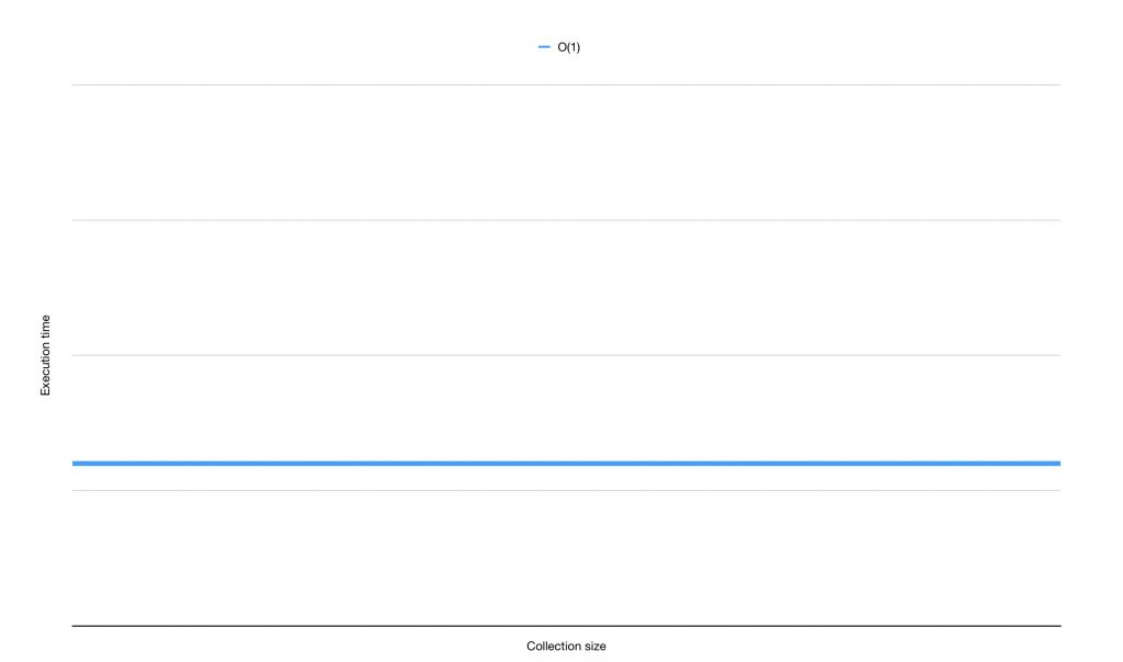
As you can see, the time needed to execute this algorithm is the same regardless of the size of the data set.

An example of an O(1) algorithm you might be familiar with is getting an element from an array using a subscript:

let array = [1, 2, 3]
array[0] // this is done in O(1)

This means that no matter how big your array is, reading a value at a certain position will always have the same performance implications.

Note that I'm not saying that "it's always fast" or "always performs well". An algorithm that is O(1) can be very slow or perform horribly. All O(1) says is that an algorithm's performance does not depend on the size of the data set it's applied to.

An algorithm that has O(1) as its complexity is considered constant. Its performance does not degrade as the data set it's applied to grows.

An example of a complexity that grows as a dataset grows is O(n). This notation communicates linear growth. The algorithm's execution time or performance degrades linearly with the size of the data set. The following graph demonstrates linear growth:

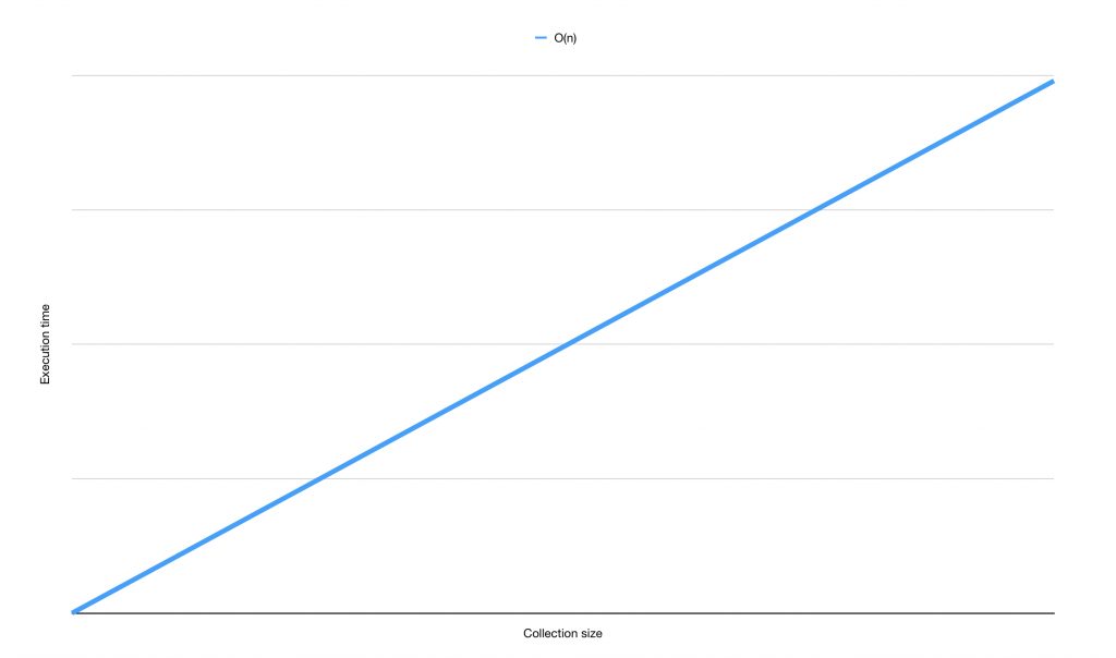
An example of a linear growth algorithm in Swift is map. Because map has to loop over all items in your array, a map is considered an algorithm with O(n) complexity. A lot of Swift's built-in functional operators have similar performance. filter, compactMap, and even first(where:) all have O(n) complexity.

If you're familiar with first(where:) it might surprise you that it's also O(n). I just explained that O(n) means that you loop over, or visit, all items in the data set once. first(where:) doesn't (have to) do this. It can return as soon as an item is found that matches the predicate used as the argument for where:

let array = ["Hello", "world", "how", "are", "you"]
var numberOfWordsChecked = 0
let threeLetterWord = array.first(where: { word in
    numberOfWordsChecked += 1
    return word.count == 3
})

print(threeLetterWord) // how
print(numberOfWordsChecked) // 3

As this code shows, we only need to loop over the array three times to find a match. Based on the rough definition I gave you earlier, you might say that this argument clearly isn't O(n) because we didn't loop over all of the elements in the array like map did.

You're not wrong! But Big O notation does not care for your specific use case. If we'd be looking for the first occurrence of the word "Big O" in that array, the algorithm would have to loop over all elements in the array and still return nil because it couldn't find a match.

Big O notation is most commonly used to depict a "worst case" or "most common" scenario. In the case of first(where:) it makes sense to assume the worst-case scenario. first(where:) is not guaranteed to find a match, and if it does, it's equally likely that the match is at the beginning or end of the data set.

Earlier, I mentioned that reading data from an array is an O(1) operation because no matter how many items the array holds, the performance is always the same. The Swift documentation writes the following about inserting items into an array:

Complexity: Reading an element from an array is O(1). Writing is O(1) unless the array's storage is shared with another array or uses a bridged NSArray instance as its storage, in which case writing is O(n), where n is the length of the array.

This is quite interesting because arrays do something special when you insert items into them. An array will usually reserve a certain amount of memory for itself. Once the array fills up, the reserved memory might not be large enough and the array will need to reserve some more memory for itself. This resizing of memory comes with a performance hit that's not mentioned in the Swift documentation. I'm pretty sure the reason for this is that the Swift core team decided to use the most common performance for array writes here rather than the worst case. It's far more likely that your array doesn't resize when you insert a new item than that it does resize.

Before I dive deeper into how you can determine the Big O of an algorithm I want to show you two more examples. This example is quadratic performance, or O(n^2):

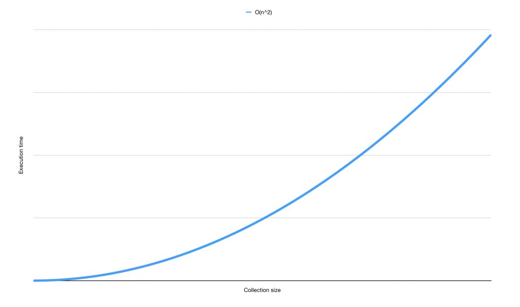
Quadratic performance is common in some simple sorting algorithms like bubble sort. A simple example of an algorithm that has quadratic performance looks like this:

let integers = (0..<5)
let squareCoords = integers.flatMap { i in 
    return integers.map { j in 
        return (i, j)
    }
}

print(squareCoords) // [(0,0), (0,1), (0,2) ... (4,2), (4,3), (4,4)]

Generating the squareCoords requires me to loop over integers using flatMap. In that flatMap, I loop over squareCoords again using a map. This means that the line return (i, j) is invoked 25 times which is equal to 5^2. Or in other words, n^2. For every element we add to the array, the time it takes to generate squareCoords grows exponentially. Creating coordinates for a 6x6 square would take 36 loops, 7x7 would take 49 loops, 8x8 takes 64 loops and so forth. I'm sure you can see why O(n^2) isn't the best performance to have.

The last common performance notation I want to show you is O(log n). As the name of this notation shows, we're dealing with a complexity that grows on a logarithmic scale. Let's look at a graph:

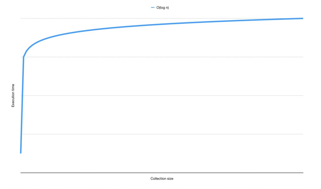
An algorithm with O(log n) complexity will often perform worse than some other algorithms for a smaller data set. However, as the data set grows and n approaches an infinite number, the algorithm's performance will degrade less and less. An example of this is a binary search. Let's assume we have a sorted array and want to find an element in it. A binary search would be a fairly efficient way of doing this:

extension RandomAccessCollection where Element: Comparable, Index == Int {
    func binarySearch(for item: Element) -> Index? {
        guard self.count > 1 else {
            if let first = self.first, first == item {
                return self.startIndex
            }  else {
                return nil
            }
        }

        let middleIndex = (startIndex + endIndex) / 2
        let middleItem = self[middleIndex]

        if middleItem < item {
            return self[index(after: middleIndex)...].binarySearch(for: item)
        } else if middleItem > item {
            return self[..<middleIndex].binarySearch(for: item)
        } else {
            return middleIndex
        }
    }
}

let words = ["Hello", "world", "how", "are", "you"].sorted()
print(words.binarySearch(for: "world")) // Optional(3)

This implementation of a binary search assumes that the input is sorted in ascending order. In order to find the requested element, it finds the middle index of the data set and compares it to the requested element. If the requested element is expected to exist before the current middle element, the array is cut in half and the first half is used to perform the same task until the requested element is found. If the requested element should come after the middle element, the second half of the array is used to perform the same task.

A search algorithm is very efficient because the number of lookups grows much slower than the size of the data set. Consider the following:

For 1 item, we need at most 1 lookup
For 2 items, we need at most 2 lookups
For 10 items, we need at most 3 lookups
For 50 items, we need at most 6 lookups
For 100 items, we need at most 7 lookups
For 1000 items, we need at most 10 lookups

Notice how going from ten to fifty items makes the data set five times bigger but the lookups only double. And going from a hundred to a thousand elements grows the data set tenfold but the number of lookups only grows by three. That's not even fifty percent more lookups for ten times the items. This is a good example of how the performance degradation of an O(log n) algorithm gets less significant as the data set increases.

Let's overlay all three graphs I've shown you so far so you can compare them.

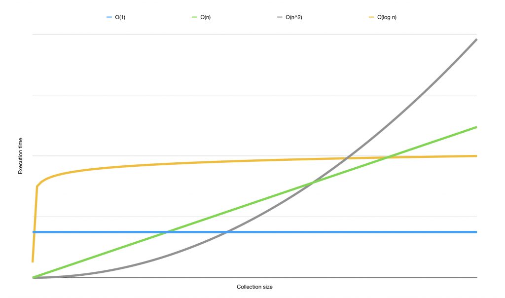
Notice how each complexity has a different curve. This makes different algorithms a good fit for different purposes. There are many more common Big O complexity notations used in programming. Take a look at this Wikipedia page to get an idea of several common complexities and to learn more about the mathematical reasoning behind Big O.

Determining the Big O notation of your code

Now that you have an idea of what Big O is, what it depicts and roughly how it's determined, I want to take a moment and help you determine the Big O complexity of code in your projects.

With enough practice, determining the Big O for an algorithm will almost become an intuition. I'm always thoroughly impressed when folks have developed this sense because I'm not even close to being able to tell Big O without carefully examining and thinking about the code at hand.

A simple way to tell the performance of code could be to look at the number of for loops in a function:

func printAll<T>(from items: [T]) {
    for item in items {
        print(item)
    }
}

This code is O(n). There's a single for loop in there and the function loops over all items from its input without ever breaking out. It's pretty clear that the performance of this function degrades linearly.

Alternatively, you could consider the following as O(1):

func printFirst<T>(_ items: [T]) {
    print(items.first)
}

There are no loops and just a single print statement. This is pretty straightforward. No matter how many items are in [T], this code will always take the same time to execute.

Here's a trickier example:

func doubleLoop<T>(over items: [T]) {
    for item in items {
        print("loop 1: \(item)")
    }

    for item in items {
        print("loop 2: \(item)")
    }
}

Ah! You might think. Two loops. So it's O(n^2) because in the example from the previous section the algorithm with two loops was O(n^2).

The difference is that the algorithm from that example had a nested loop that iterated over the same data as the outer loop. In this case, the loops are alongside each other which means that the execution time is twice the number of elements in the array. Not the number of elements in the array squared. For that reason, this example can be considered O(2n). This complexity is often shortened to O(n) because the performance degrades linearly. It doesn't matter that we loop over the data set twice.

Let's take a look at an example of a loop that's shown in Cracking the Coding Interview that had me scratching my head for a while:

func printPairs(for integers: [Int]) {
    for (idx, i) in integers.enumerated() {
        for j in integers[idx...] {
            print((i, j))
        }
    }
}

The code above contains a nested loop, so it immediately looks like O(n^2). But look closely. We don't loop over the entire data set in the nested loop. Instead, we loop over a subset of elements. As the outer loop progresses, the work done in the inner loop diminishes. If I write down the printed lines for each iteration of the outer loop it'd look a bit like this if the input is [1, 2, 3]:

(1, 1) (1, 2) (1, 3)
(2, 2) (2, 3)
(3, 3)

If we'd add one more element to the input, we'd need four more loops:

(1, 1) (1, 2) (1, 3) (1, 4)
(2, 2) (2, 3) (2, 4)
(3, 3) (3, 4)
(4, 4)

Based on this, we can say that the outer loop executes n times. It's linear to the number of items in the array. The inner loop runs roughly half of n on average for each time the outer loop runs. The first time it runs n times, then n-1, then n-2 and so forth. So one might say that the runtime for this algorithm is O(n * n / 2) which is the same as O(n^2 / 2) and similar to how we simplified O(2n) to O(n), it's normal to simplify O(n^2 / 2) to O(n^2).

The reason you can simplify O(n^2 / 2) to O(n^2) is because Big O is used to describe a curve, not the exact performance. If you'd plot graphs for both formulas, you'd find that the curves look similar. Dividing by two simply doesn’t impact the performance degradation of this algorithm in a significant way. For that reason, it's preferred to use the simpler Big O notation instead of the complex detailed one because it communicates the complexity of the algorithm much clearer.

While you may have landed on O(n^2) by seeing the two nested for loops immediately, it's important to understand the reasoning behind such a conclusion too because there’s a little bit more to it than just counting loops.

In summary

Big O is one of those things that you have to practice often to master it. I have covered a handful of common Big O notations in this week's post, and you saw how those notations can be derived from looking at code and reasoning about it. Some developers have a sense of Big O that's almost like magic, they seem to just know all of the patterns and can uncover them in seconds. Others, myself included, need to spend more time analyzing and studying to fully understand the Big O complexity of a given algorithm.

If you want to brush up on your Big O skills, I can only recommend practice. Tons and tons of practice. And while it might be a bit much to buy a whole book for a small topic, I like the way Cracking the Coding Interview covers Big O. It has been helpful for me. There was a very good talk at WWDC 2018 about algorithms by Dave Abrahams too. You might want to check that out. It's really good.

If you've got any questions or feedback about this post, don't hesitate to reach out on Twitter.